Friday, June 24, 2005
Rule 16: StatusBar
Use the Status bar to report information back to the user whilst code is being executed.
For example, if several files or database queries are being run, then
will display a message on the status bar.
Will remove the value on the status bar.
However, we are then back with the issue of nested calls.
Its much better to create two utility functions, with the call, PushStatusMessage, and PopStatusMessage that creates a stack of status messages.
For example, if several files or database queries are being run, then
Application.StatusBar = "Loading file 1 ..."
will display a message on the status bar.
Application.StatusBar = False
Will remove the value on the status bar.
However, we are then back with the issue of nested calls.
Its much better to create two utility functions, with the call, PushStatusMessage, and PopStatusMessage that creates a stack of status messages.
Private Const MaxStatusMessage As Integer = 100
Dim StatusMessages(MaxStatusMessage) As String
Dim StatusMessageCount As Integer

Public Sub PushStatusMessage(message As String)
    If StatusMessageCount = MaxStatusMessage Then
        MsgBox "Status message stack is full"
        Exit Sub
    End If
    StatusMessages(StatusMessageCount) = message
    StatusMessageCount = StatusMessageCount + 1
    Application.StatusBar = message
End Sub

Public Sub PopStatusMessage()
    If StatusMessageCount = 0 Then
        'MsgBox "Status message stack is empty"
        Exit Sub
    End If
    StatusMessageCount = StatusMessageCount - 1
    If StatusMessageCount = 0 Then
        Application.StatusBar = False
    Else
        Application.StatusBar = StatusMessages(StatusMessageCount - 1)
    End If
End Sub

Public Sub Test()
    PushStatusMessage ("Test 1")
    PushStatusMessage ("Test 2")
    PopStatusMessage
    PopStatusMessage
End Sub
Rule 15: Screen Updating
There is a flag Application.ScreenUpdating that can be set to True or False.
Setting it to False whilst building up code makes the application run faster.
However, in order to write code where you can nest calls means that each subroutine has to remember the state of the flag, and reset it when you exit the subroutine. If there is an early exit, or exception, the flag will not be restored.
One possible solution is a utility subroutine that keeps a stack of the values. Its certainly easier than maintaining flags by hand.
However, there is another approach. Just set the flag in the button code. That will always be at the top level so only one flag is needed. Just make sure its caught in the case of errors.
Private Sub CommandButton1_Click()
    Dim su As Boolean
    su = Application.ScreenUpdating
    Application.ScreenUpdating = False
On Error GoTo finish
    ' Do some work here
    Application.ScreenUpdating = su
    Exit Sub
finish:
    Application.ScreenUpdating = su
End Sub
Tuesday, June 21, 2005
Trick 1: Reconciliation
Quite often there is a need to do quick reconcilliations between two different systems.
Take a simple example. You are converting from system A to system B and need to make sure all the items are loaded into system B, and that a calculated value agrees.
How does one do this in Excel?
First we need to load the data into Excel. This can be done in various ways, but ADODB is probably the best.
The data needs to be loaded in a certain form, and this diagram illustrates what is required.
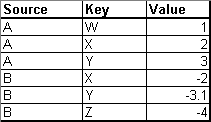
The first column contains the name of the source system. The second column contains the key we need to use to match. The last column contains the calculated value. We load up all the rows from system A, then append the rows from system B.
When we load the calculated value from the second system, we negate the number. More on this later.
Now we can proceed to phase two. We select all the data, and then build a pivot table from the results. The source goes in the column headers. The key goes in the row, and the calculated value goes in the data area.
The pivot table will now look like this.
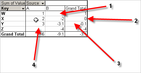
So what do we have. Anything with a blank in the A or B column means a missing or extra item. When there are two items, but a non zero grand total for the row, this grand total shows the difference.
1. There is a blank in the B column. That means an item in system A doesn't exist in system B
2. We have an item in both, and a zero grand total. That means a perfect match.
3. We have an item in both, but the values are different. 3 and 3.1 or a difference of 0.1
4. A blank in column A means an item in system B exists, where as it doesn't exists in system A
Its as quick as that.
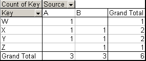
This shows what happens if you put the key or source in the data area. Normally a key would be a string, so it won't sum the data, it counts it. Here we can quickly see anything with a 1 in the data illustrates a missing value. The grand totals of the columns show the number of items from each source.
If you were doing this as part of a conversion, it pays to automate the process. For example, you could build some macros that download all the data, then build the pivot table.
Once the pivot table is built, you can write a macro that hides the good data, just displaying the bad or vice versa.
If you do this, another enhancement is to add on a name to sign off the differences. Then all you need to do as part of a big bang conversion is to run the reconciliation, filter the good items out. That then needs to be signed off by the business, and filed.
This is probably the best Excel trick I have come across. Its not obvious at all that Excel can do things like this without doing a lot of work.
Thanks Dom!
Take a simple example. You are converting from system A to system B and need to make sure all the items are loaded into system B, and that a calculated value agrees.
How does one do this in Excel?
First we need to load the data into Excel. This can be done in various ways, but ADODB is probably the best.
The data needs to be loaded in a certain form, and this diagram illustrates what is required.

The first column contains the name of the source system. The second column contains the key we need to use to match. The last column contains the calculated value. We load up all the rows from system A, then append the rows from system B.
When we load the calculated value from the second system, we negate the number. More on this later.
Now we can proceed to phase two. We select all the data, and then build a pivot table from the results. The source goes in the column headers. The key goes in the row, and the calculated value goes in the data area.
The pivot table will now look like this.

So what do we have. Anything with a blank in the A or B column means a missing or extra item. When there are two items, but a non zero grand total for the row, this grand total shows the difference.
1. There is a blank in the B column. That means an item in system A doesn't exist in system B
2. We have an item in both, and a zero grand total. That means a perfect match.
3. We have an item in both, but the values are different. 3 and 3.1 or a difference of 0.1
4. A blank in column A means an item in system B exists, where as it doesn't exists in system A
Its as quick as that.

This shows what happens if you put the key or source in the data area. Normally a key would be a string, so it won't sum the data, it counts it. Here we can quickly see anything with a 1 in the data illustrates a missing value. The grand totals of the columns show the number of items from each source.
If you were doing this as part of a conversion, it pays to automate the process. For example, you could build some macros that download all the data, then build the pivot table.
Once the pivot table is built, you can write a macro that hides the good data, just displaying the bad or vice versa.
If you do this, another enhancement is to add on a name to sign off the differences. Then all you need to do as part of a big bang conversion is to run the reconciliation, filter the good items out. That then needs to be signed off by the business, and filed.
This is probably the best Excel trick I have come across. Its not obvious at all that Excel can do things like this without doing a lot of work.
Thanks Dom!
Monday, June 20, 2005
Rule 14: Give Modules meaningful names
Module1 is not a meaningful name. Point made.
Rule 13: VBA Formulas versus Worksheet formulas
Quite often there is a choice. Write a formula in the worksheet, or produce some VBA code. How does one make the decision?
If there is conditional logic, then the first port of call is a VBA function. Its very difficult to read conditional logic in a worksheet formula, and they also tend to be quite long.
If the partial results are meaningful, then put these on the spreadsheet and break the formulas down in their component parts.
For example, if profit and loss is made up of different parts, cash, mark to market, transaction costs, fees etc, then a column for each of the parts makes sense. Then they can be totaled in the profit and loss column. If necessary, the other columns can be hidden. It makes debugging and analysis easier.
Putting the formula into VBA also gives a name to what the formula intends to achieve. ie. =B2+C2+D2 doesn't convey much meaning. =Cash(A2) + MarkToMarket(A2) + TCosts(A2) + Fees(A2) makes a lot more sense, even if you have to dig around for the details.
Putting the formulas into VBA also enables their definition to be in one place and one place only. ie. Code it once, not cut and paste the formula everywhere. The code can then be moved out to an XLA an centralised.
Rule 12: The macro recorder produces bad code
The macro recorder produces bad code. Cut and paste, select / selection has been covered. It does other things too that aren't particularly good.
For example, it doesn't know about named ranges. As such it uses A1 style references all the time.
These should be cleaned up.
The code is very much a stream of conciousness type of approach to coding. Its much better to put some structure to the code.
Break the macro down into subroutines.
Rename the MacroN name of the recording to something that makes sense.
Remove the select / selection from the code
Remove the copy / paste constructs.
Think about any loops that make the code easier.
What about variables? Should things be declared as variables?
Rule 11: Hungarian Notation is bad
Its quite easy to show why Hungarian notation is bad, and its a point that is often missed in the religious wars on the subject.
If you were designing a database or even an Excel spreadsheet, it would be an awful spreadsheet if the user had to enter the same number in lots of cells.
The principle that should be followed is to have one cell storing the data and refer to that cell. ie. Store the data once.
Hungarian notation goes against that priciple. Instead of storing the type of something in one place, its stores it everywhere it is used.
Here the type, an integer counter is stored and repeated everytime the variable is used instead of once, in the dim statement.
If you want to change the type to a long, you have to change the dim, and everytime its used. If you code is used by others, its a real problem. Just your own code is bad enough.
Instead just do this.
Then you can change the type in once place and one place only.
The intent comes from the comment.
If you were designing a database or even an Excel spreadsheet, it would be an awful spreadsheet if the user had to enter the same number in lots of cells.
The principle that should be followed is to have one cell storing the data and refer to that cell. ie. Store the data once.
Hungarian notation goes against that priciple. Instead of storing the type of something in one place, its stores it everywhere it is used.
Dim icRow as Integer
...
icRow = icRow + 1
...
Here the type, an integer counter is stored and repeated everytime the variable is used instead of once, in the dim statement.
If you want to change the type to a long, you have to change the dim, and everytime its used. If you code is used by others, its a real problem. Just your own code is bad enough.
Instead just do this.
Dim row as Integer 'index to the rows in the range
...
row = row + 1
...
Then you can change the type in once place and one place only.
The intent comes from the comment.
Rule 10: Copy and Paste in VBA is evil
Just like select and selection, copy and paste in VBA codes is also evil. Its a side effect problem again and it can be avoided.
Here is some typical generated code.
Taking out the select, we still have a problem.
It still has a side effect of putting some values in the clipboard.
Here is some code that does the job without any side effects.
Shorter and side effect free.
It also means the user isn't surprised if they run a macro and then try and paste what they thought was in the clipboard into a new range or cell.
Here is some typical generated code.
    Range("A13:B23").Select
    Selection.Copy
    Range("A26:B36").Select
    ActiveSheet.Paste
Taking out the select, we still have a problem.
    Range("A13:B23").Copy
    Range("A26:B36").Paste
It still has a side effect of putting some values in the clipboard.
Here is some code that does the job without any side effects.
Range("A26:B36").value = Range("A13:B23").value
Shorter and side effect free.
It also means the user isn't surprised if they run a macro and then try and paste what they thought was in the clipboard into a new range or cell.
Rule 9: Select is evil
The macro recorder likes producing this sort of code.
This is evil.
Here is why.
Bundle the code up in a subroutine
Seems reasonable.
However lets say we have another subroutine
The idea is that we want to set the colour of the sells A14:B20, and highlight E13:G16.
Sorry, it doesn't work. You cannot nest the calls, because of the .Select statement. It changes the selection and is a side effect of the call to Highlight. The end result is you cannot decompose your subroutines in this way.
The code should be this
This is now side effect free.
ie. Remove all the .select / .selection from the code.
    Range("E13:G16").Select
    Selection.Font.Bold = True
This is evil.
Here is why.
Bundle the code up in a subroutine
Public Sub Highlight()
    Range("E13:G16").Select
    Selection.Font.Bold = True
End Sub
Seems reasonable.
However lets say we have another subroutine
Public Sub FormatCells()
    Range ("A14:B20").Select
    Highlight()
    With Selection.Interior
        .ColorIndex = 7
        .Pattern = xlSolid
    End With
End Sub
The idea is that we want to set the colour of the sells A14:B20, and highlight E13:G16.
Sorry, it doesn't work. You cannot nest the calls, because of the .Select statement. It changes the selection and is a side effect of the call to Highlight. The end result is you cannot decompose your subroutines in this way.
The code should be this
Public Sub Highlight()
    Range("E13:G16").Selection.Font.Bold = True
End Sub

Public Sub FormatCells()
    Highlight()
    With Range ("A14:B20").Interior
        .ColorIndex = 7
        .Pattern = xlSolid
    End With
End Sub
This is now side effect free.
ie. Remove all the .select / .selection from the code.
Rule 8: Formatting
Be consistent with formating.
On the colour front, pick pastel colours, they seem to work well.
Use boxes to mark areas with borders. Outside borders with double thickness lines,
inside borders with single
Pick a consistent colour for cells that can be inputed by the user. Combine this with protection.
Highlight error conditions with non-pastel colours. For example, bold white on a red background.
Use conditional formatting to set the colours were relevant. For example with an arbitrage situation, there are three states. Not worth doing the deal, a cheaper sythetic deal, and an outright arbitrage. That's three colours. The first is probably the same as the background, the second pastel, the last primary.
Rule 7: Version Page
Put in a page that gets hidden as part of the debug on / debug off macro. This should have a data, a modifier, and a record of the changes made to the code for the spreadsheet.
Standardise on the name such as Versions

Standardise on the name such as Versions

Rule 6: Database or Excel
Use Excel where it has strengths. Sumarising data, performing calculations on data.
Use a Database where it has strengths, capturing large amounts of dat.a
A clear example is keeping historical prices. Don't use Excel, use a database an retrieve the data or a summary of the data when needed.
Use a Database where it has strengths, capturing large amounts of dat.a
A clear example is keeping historical prices. Don't use Excel, use a database an retrieve the data or a summary of the data when needed.
Rule 5: Debug On / Debug Off
Create a debug on and debug off macro.
This macro hides all the sheets the user doesn't need to see, or vice versa.
It can also turn protection on and off if that is being used.
If there is special formating on some sheet, it may put the grid lines back, enable stasus bars etc that are needed for development.
Here is an example.
This macro hides all the sheets the user doesn't need to see, or vice versa.
It can also turn protection on and off if that is being used.
If there is special formating on some sheet, it may put the grid lines back, enable stasus bars etc that are needed for development.
Here is an example.
Option Explicit

Public Sub Display(b As Boolean)
    Sheets("Parameters").Visible = b
    Sheets("CurrentData").Visible = b
    Sheets("DeltaData").Visible = b
    Sheets("AbsoluteData").Visible = b
End Sub

Public Sub Test()
    Display (True)
End Sub

Public Sub Prod()
    Display (False)
    Application.ScreenUpdating = True
    Application.Calculation = xlCalculationAutomatic
End Sub
Rule 4: Parameter sheet
Create a sheet called parameters. In this sheet set up names down the left hand side, and values in the next column. Then names can be created for the cells on the right hand side. These form the parameters to be used elsewhere.
A typical example would be the name, password and database to use in a database connection.
This sheet should be hidden as part of the debug on / debug off macro
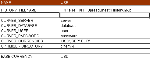
A typical example would be the name, password and database to use in a database connection.
This sheet should be hidden as part of the debug on / debug off macro

Rule 3: Data Access
Don't use Query tables. They tend to leave lots of copies of themselves around. It can be quite difficult editing the queries.
Instead, write some generic ADODB code that uses a record set. A query can then just be a worksheet, an SQL string, and a reference to the parameters stored on a sheet.
The query clears the worksheet, runs the query, returns the data to the worksheet, and names the results as a range with the same name as the worksheet.
The worksheets should probably be hidden with the debug on / debug off macro.
The key to the data should be the first column to help with vlookup working as a function.
The generic code should be split out as an XLA file and referenced in.
Rule 2: Named Ranges
Its a pretty strong rule that a block of cells should have a name.
Its not so clear that each column should have a range name. If you do create the names in the column headings it can make formulas easer to understand. However, it does create a lot of names. If the names are similar to others, it becomes difficult to untangle them.
Its not so clear that each column should have a range name. If you do create the names in the column headings it can make formulas easer to understand. However, it does create a lot of names. If the names are similar to others, it becomes difficult to untangle them.
Rule 1: Option Explicit
In your VBA code, always put option explicit as the first line. This will stop code running with variables that haven't been declared.
Sunday, June 12, 2005
Aims
I'm putting this micro blog together to record thoughts about using Excel, neat tricks, and in particular to form a set of coding standards and ideas on how to use Excel, particularly in a financial environment.
Nick
Nick
Subscribe to Posts [Atom]